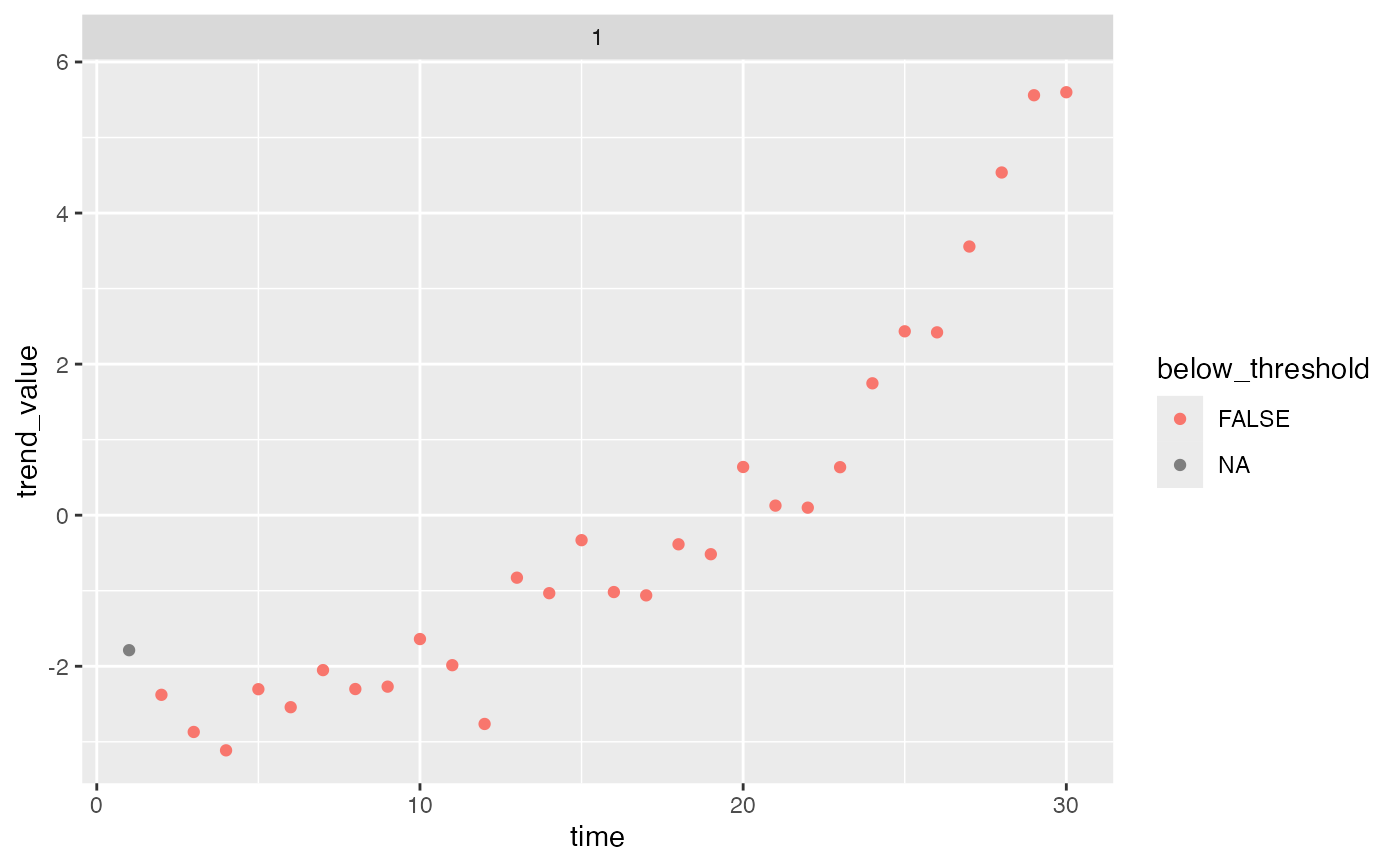
Find outlying "black swan" jumps in trends
find_swans(rotated_modelfit, threshold = 0.01, plot = FALSE)Arguments
- rotated_modelfit
Output from
rotate_trends().- threshold
A probability threshold below which to flag trend events as extreme
- plot
Logical: should a plot be made?
Value
Prints a ggplot2 plot if plot = TRUE; returns a data frame indicating the
probability that any given point in time represents a "black swan" event
invisibly.
References
Anderson, S.C., Branch, T.A., Cooper, A.B., and Dulvy, N.K. 2017. Black-swan events in animal populations. Proceedings of the National Academy of Sciences 114(12): 3252–3257. https://doi.org/10.1073/pnas.1611525114
Examples
set.seed(1)
s <- sim_dfa(num_trends = 1, num_ts = 3, num_years = 30)
s$y_sim[1, 15] <- s$y_sim[1, 15] - 6
plot(s$y_sim[1, ], type = "o")
abline(v = 15, col = "red")
 # only 1 chain and 250 iterations used so example runs quickly:
m <- fit_dfa(y = s$y_sim, num_trends = 1, iter = 50, chains = 1, nu_fixed = 2)
#>
#> SAMPLING FOR MODEL 'dfa' NOW (CHAIN 1).
#> Chain 1:
#> Chain 1: Gradient evaluation took 1.9e-05 seconds
#> Chain 1: 1000 transitions using 10 leapfrog steps per transition would take 0.19 seconds.
#> Chain 1: Adjust your expectations accordingly!
#> Chain 1:
#> Chain 1:
#> Chain 1: WARNING: There aren't enough warmup iterations to fit the
#> Chain 1: three stages of adaptation as currently configured.
#> Chain 1: Reducing each adaptation stage to 15%/75%/10% of
#> Chain 1: the given number of warmup iterations:
#> Chain 1: init_buffer = 3
#> Chain 1: adapt_window = 20
#> Chain 1: term_buffer = 2
#> Chain 1:
#> Chain 1: Iteration: 1 / 50 [ 2%] (Warmup)
#> Chain 1: Iteration: 5 / 50 [ 10%] (Warmup)
#> Chain 1: Iteration: 10 / 50 [ 20%] (Warmup)
#> Chain 1: Iteration: 15 / 50 [ 30%] (Warmup)
#> Chain 1: Iteration: 20 / 50 [ 40%] (Warmup)
#> Chain 1: Iteration: 25 / 50 [ 50%] (Warmup)
#> Chain 1: Iteration: 26 / 50 [ 52%] (Sampling)
#> Chain 1: Iteration: 30 / 50 [ 60%] (Sampling)
#> Chain 1: Iteration: 35 / 50 [ 70%] (Sampling)
#> Chain 1: Iteration: 40 / 50 [ 80%] (Sampling)
#> Chain 1: Iteration: 45 / 50 [ 90%] (Sampling)
#> Chain 1: Iteration: 50 / 50 [100%] (Sampling)
#> Chain 1:
#> Chain 1: Elapsed Time: 0.053 seconds (Warm-up)
#> Chain 1: 0.027 seconds (Sampling)
#> Chain 1: 0.08 seconds (Total)
#> Chain 1:
#> Warning: There were 24 divergent transitions after warmup. See
#> https://mc-stan.org/misc/warnings.html#divergent-transitions-after-warmup
#> to find out why this is a problem and how to eliminate them.
#> Warning: Examine the pairs() plot to diagnose sampling problems
#> Warning: The largest R-hat is 2.1, indicating chains have not mixed.
#> Running the chains for more iterations may help. See
#> https://mc-stan.org/misc/warnings.html#r-hat
#> Warning: Bulk Effective Samples Size (ESS) is too low, indicating posterior means and medians may be unreliable.
#> Running the chains for more iterations may help. See
#> https://mc-stan.org/misc/warnings.html#bulk-ess
#> Warning: Tail Effective Samples Size (ESS) is too low, indicating posterior variances and tail quantiles may be unreliable.
#> Running the chains for more iterations may help. See
#> https://mc-stan.org/misc/warnings.html#tail-ess
#> Inference for the input samples (1 chains: each with iter = 25; warmup = 12):
#>
#> Q5 Q50 Q95 Mean SD Rhat Bulk_ESS Tail_ESS
#> x[1,1] -1.2 -1.1 -1.0 -1.1 0.1 1.45 4 13
#> x[1,2] -0.9 -0.8 -0.8 -0.8 0.1 1.71 4 13
#> x[1,3] -1.1 -1.1 -0.9 -1.0 0.1 0.93 13 13
#> x[1,4] -1.7 -1.6 -1.5 -1.6 0.1 1.01 10 13
#> x[1,5] -2.1 -2.0 -1.9 -2.0 0.1 0.97 12 13
#> x[1,6] -1.3 -1.1 -1.0 -1.1 0.1 1.05 9 13
#> x[1,7] -0.8 -0.7 -0.5 -0.6 0.1 1.09 10 13
#> x[1,8] -1.6 -1.5 -1.3 -1.4 0.1 0.98 13 13
#> x[1,9] -1.1 -1.0 -0.8 -1.0 0.1 1.15 13 13
#> x[1,10] -1.1 -1.0 -0.9 -1.0 0.1 1.19 7 13
#> x[1,11] -0.9 -0.8 -0.6 -0.8 0.1 1.09 13 13
#> x[1,12] -1.6 -1.4 -1.3 -1.4 0.1 1.32 5 13
#> x[1,13] -0.4 -0.3 -0.2 -0.3 0.1 1.19 13 13
#> x[1,14] -0.3 -0.2 0.0 -0.2 0.1 1.02 13 13
#> x[1,15] -0.4 -0.2 0.0 -0.2 0.1 0.94 13 13
#> x[1,16] -0.5 -0.2 -0.1 -0.3 0.1 1.49 13 13
#> x[1,17] -0.8 -0.7 -0.4 -0.6 0.2 1.71 13 13
#> x[1,18] -0.3 -0.2 0.0 -0.2 0.1 2.07 13 13
#> x[1,19] -0.2 -0.1 0.1 -0.1 0.1 1.91 13 13
#> x[1,20] 0.2 0.3 0.6 0.4 0.1 1.16 13 13
#> x[1,21] 0.8 0.9 1.2 0.9 0.1 1.21 13 13
#> x[1,22] 0.5 0.7 1.0 0.7 0.1 1.34 6 13
#> x[1,23] 0.5 0.7 0.9 0.7 0.1 1.24 9 13
#> x[1,24] 0.8 0.9 1.2 1.0 0.1 1.24 13 13
#> x[1,25] 0.7 0.8 1.1 0.8 0.1 1.21 7 13
#> x[1,26] 1.3 1.4 1.6 1.4 0.1 1.16 13 13
#> x[1,27] 2.1 2.2 2.4 2.2 0.1 1.09 13 13
#> x[1,28] 2.6 2.7 3.0 2.7 0.1 1.13 13 13
#> x[1,29] 2.7 2.7 3.0 2.8 0.1 1.18 9 13
#> x[1,30] 2.1 2.2 2.5 2.3 0.1 1.60 13 13
#> Z[1,1] -0.7 -0.6 -0.5 -0.6 0.1 1.87 4 13
#> Z[2,1] -0.8 -0.7 -0.6 -0.7 0.1 1.16 13 13
#> Z[3,1] -0.8 -0.7 -0.5 -0.7 0.1 1.20 6 13
#> log_lik[1] -0.2 -0.2 -0.2 -0.2 0.0 1.21 6 13
#> log_lik[2] -0.3 -0.2 -0.2 -0.2 0.1 0.96 10 13
#> log_lik[3] -0.4 -0.3 -0.2 -0.3 0.1 1.74 4 13
#> log_lik[4] -0.9 -0.6 -0.5 -0.7 0.2 2.07 4 13
#> log_lik[5] -0.4 -0.2 -0.2 -0.3 0.1 0.97 13 7
#> log_lik[6] -0.4 -0.2 -0.2 -0.2 0.1 1.38 5 7
#> log_lik[7] -0.3 -0.3 -0.2 -0.3 0.1 1.71 4 13
#> log_lik[8] -0.3 -0.2 -0.2 -0.2 0.1 2.12 12 7
#> log_lik[9] -0.6 -0.3 -0.2 -0.3 0.1 1.13 10 7
#> log_lik[10] -0.3 -0.2 -0.2 -0.2 0.1 1.39 6 13
#> log_lik[11] -0.3 -0.2 -0.1 -0.2 0.1 1.12 9 13
#> log_lik[12] -0.3 -0.2 -0.2 -0.2 0.1 0.96 13 7
#> log_lik[13] -0.9 -0.6 -0.3 -0.6 0.2 1.58 4 13
#> log_lik[14] -1.5 -0.8 -0.5 -0.9 0.5 1.46 13 13
#> log_lik[15] -1.2 -1.0 -0.3 -0.9 0.3 1.19 9 13
#> log_lik[16] -0.3 -0.3 -0.2 -0.3 0.1 1.18 7 13
#> log_lik[17] -0.3 -0.2 -0.2 -0.2 0.1 1.01 10 13
#> log_lik[18] -0.3 -0.2 -0.2 -0.2 0.0 0.94 13 13
#> log_lik[19] -0.6 -0.5 -0.3 -0.5 0.1 1.08 12 13
#> log_lik[20] -0.9 -0.7 -0.4 -0.7 0.2 1.03 10 13
#> log_lik[21] -0.8 -0.6 -0.4 -0.6 0.2 1.07 11 7
#> log_lik[22] -0.3 -0.2 -0.2 -0.2 0.0 1.32 5 13
#> log_lik[23] -0.3 -0.2 -0.1 -0.2 0.1 1.16 7 13
#> log_lik[24] -0.3 -0.2 -0.1 -0.2 0.1 1.09 13 7
#> log_lik[25] -0.6 -0.4 -0.3 -0.4 0.1 1.91 9 7
#> log_lik[26] -0.3 -0.2 -0.2 -0.2 0.1 1.12 7 7
#> log_lik[27] -0.4 -0.2 -0.2 -0.2 0.1 0.99 8 7
#> log_lik[28] -0.3 -0.2 -0.2 -0.2 0.0 0.95 13 7
#> log_lik[29] -0.3 -0.2 -0.2 -0.2 0.1 1.38 8 7
#> log_lik[30] -0.4 -0.2 -0.2 -0.2 0.1 1.01 8 7
#> log_lik[31] -0.3 -0.2 -0.2 -0.2 0.1 0.96 13 7
#> log_lik[32] -0.4 -0.3 -0.2 -0.3 0.1 2.12 10 7
#> log_lik[33] -0.3 -0.2 -0.1 -0.2 0.1 1.10 11 7
#> log_lik[34] -0.3 -0.2 -0.2 -0.2 0.0 1.16 13 13
#> log_lik[35] -0.5 -0.2 -0.2 -0.3 0.1 1.71 4 13
#> log_lik[36] -0.6 -0.3 -0.2 -0.4 0.1 1.15 11 13
#> log_lik[37] -1.2 -1.1 -0.8 -1.1 0.1 1.15 13 13
#> log_lik[38] -1.0 -0.9 -0.6 -0.8 0.2 1.30 13 7
#> log_lik[39] -1.2 -1.0 -0.7 -0.9 0.2 1.21 13 7
#> log_lik[40] -1.0 -0.7 -0.6 -0.7 0.2 1.27 7 13
#> log_lik[41] -0.7 -0.5 -0.3 -0.5 0.2 1.39 13 13
#> log_lik[42] -0.6 -0.3 -0.2 -0.3 0.1 1.10 9 13
#> log_lik[43] -18.5 -17.5 -15.2 -17.0 1.3 0.92 13 13
#> log_lik[44] -0.7 -0.5 -0.3 -0.5 0.2 1.14 13 13
#> log_lik[45] -0.6 -0.3 -0.2 -0.4 0.1 1.02 13 13
#> log_lik[46] -0.6 -0.4 -0.3 -0.4 0.1 1.27 13 13
#> log_lik[47] -0.4 -0.3 -0.2 -0.3 0.1 1.33 13 13
#> log_lik[48] -0.5 -0.3 -0.2 -0.3 0.1 1.27 13 13
#> log_lik[49] -0.3 -0.2 -0.2 -0.2 0.0 1.19 13 13
#> log_lik[50] -0.3 -0.2 -0.2 -0.2 0.0 1.71 4 13
#> log_lik[51] -0.3 -0.2 -0.2 -0.2 0.1 1.00 13 13
#> log_lik[52] -0.3 -0.2 -0.2 -0.2 0.0 0.98 13 7
#> log_lik[53] -0.3 -0.2 -0.2 -0.2 0.1 1.91 13 7
#> log_lik[54] -0.4 -0.2 -0.2 -0.3 0.1 1.74 13 7
#> log_lik[55] -0.2 -0.2 -0.1 -0.2 0.0 0.92 11 13
#> log_lik[56] -0.4 -0.3 -0.2 -0.3 0.1 1.71 13 13
#> log_lik[57] -0.2 -0.2 -0.2 -0.2 0.0 0.95 13 13
#> log_lik[58] -0.2 -0.2 -0.1 -0.2 0.0 1.00 9 7
#> log_lik[59] -0.4 -0.3 -0.2 -0.3 0.1 1.16 10 13
#> log_lik[60] -0.3 -0.2 -0.2 -0.2 0.0 0.93 13 13
#> log_lik[61] -0.4 -0.2 -0.2 -0.2 0.1 1.38 11 7
#> log_lik[62] -0.3 -0.2 -0.2 -0.2 0.0 1.08 9 7
#> log_lik[63] -0.2 -0.2 -0.2 -0.2 0.0 0.93 13 13
#> log_lik[64] -0.9 -0.6 -0.5 -0.6 0.1 1.32 13 7
#> log_lik[65] -0.3 -0.2 -0.2 -0.2 0.1 1.49 5 7
#> log_lik[66] -0.3 -0.2 -0.2 -0.2 0.0 1.58 6 13
#> log_lik[67] -0.4 -0.2 -0.2 -0.3 0.1 1.47 13 7
#> log_lik[68] -0.2 -0.2 -0.2 -0.2 0.0 1.09 7 7
#> log_lik[69] -0.2 -0.2 -0.2 -0.2 0.0 0.95 9 13
#> log_lik[70] -0.4 -0.3 -0.2 -0.3 0.1 1.49 7 13
#> log_lik[71] -0.3 -0.2 -0.2 -0.2 0.0 1.37 5 13
#> log_lik[72] -0.2 -0.2 -0.1 -0.2 0.0 1.04 9 13
#> log_lik[73] -0.3 -0.2 -0.2 -0.2 0.0 1.10 9 13
#> log_lik[74] -0.6 -0.4 -0.3 -0.5 0.1 2.12 4 13
#> log_lik[75] -0.5 -0.3 -0.3 -0.3 0.1 0.94 9 13
#> log_lik[76] -0.4 -0.2 -0.2 -0.3 0.1 1.49 4 13
#> log_lik[77] -0.4 -0.3 -0.2 -0.3 0.1 1.25 6 13
#> log_lik[78] -0.5 -0.2 -0.2 -0.3 0.1 1.07 7 13
#> log_lik[79] -0.5 -0.2 -0.2 -0.3 0.1 1.21 5 13
#> log_lik[80] -0.3 -0.2 -0.2 -0.2 0.1 0.94 13 13
#> log_lik[81] -0.4 -0.2 -0.2 -0.2 0.1 1.05 6 13
#> log_lik[82] -0.4 -0.2 -0.2 -0.2 0.1 1.00 8 13
#> log_lik[83] -0.4 -0.2 -0.2 -0.2 0.1 1.00 11 13
#> log_lik[84] -0.6 -0.2 -0.2 -0.3 0.2 1.05 8 7
#> log_lik[85] -0.5 -0.2 -0.2 -0.3 0.1 1.38 5 13
#> log_lik[86] -0.9 -0.4 -0.2 -0.5 0.3 1.09 9 13
#> log_lik[87] -0.8 -0.2 -0.2 -0.4 0.3 1.19 8 7
#> log_lik[88] -0.7 -0.4 -0.2 -0.4 0.2 1.25 5 13
#> log_lik[89] -1.9 -1.2 -0.6 -1.2 0.4 1.49 5 13
#> log_lik[90] -1.6 -0.9 -0.5 -0.9 0.4 1.18 9 13
#> xstar[1,1] -11.2 1.7 3.8 -0.2 7.0 1.38 6 13
#> sigma[1] 0.5 0.5 0.5 0.5 0.0 0.94 11 13
#> lp__ -45.8 -41.5 -39.6 -41.9 2.1 1.74 9 7
#>
#> For each parameter, Bulk_ESS and Tail_ESS are crude measures of
#> effective sample size for bulk and tail quantities respectively (an ESS > 100
#> per chain is considered good), and Rhat is the potential scale reduction
#> factor on rank normalized split chains (at convergence, Rhat <= 1.05).
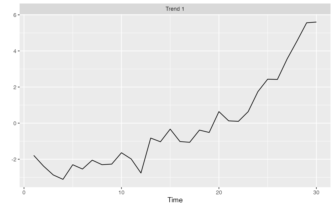
r <- rotate_trends(m)
p <- plot_trends(r) #+ geom_vline(xintercept = 15, colour = "red")
print(p)
# only 1 chain and 250 iterations used so example runs quickly:
m <- fit_dfa(y = s$y_sim, num_trends = 1, iter = 50, chains = 1, nu_fixed = 2)
#>
#> SAMPLING FOR MODEL 'dfa' NOW (CHAIN 1).
#> Chain 1:
#> Chain 1: Gradient evaluation took 1.9e-05 seconds
#> Chain 1: 1000 transitions using 10 leapfrog steps per transition would take 0.19 seconds.
#> Chain 1: Adjust your expectations accordingly!
#> Chain 1:
#> Chain 1:
#> Chain 1: WARNING: There aren't enough warmup iterations to fit the
#> Chain 1: three stages of adaptation as currently configured.
#> Chain 1: Reducing each adaptation stage to 15%/75%/10% of
#> Chain 1: the given number of warmup iterations:
#> Chain 1: init_buffer = 3
#> Chain 1: adapt_window = 20
#> Chain 1: term_buffer = 2
#> Chain 1:
#> Chain 1: Iteration: 1 / 50 [ 2%] (Warmup)
#> Chain 1: Iteration: 5 / 50 [ 10%] (Warmup)
#> Chain 1: Iteration: 10 / 50 [ 20%] (Warmup)
#> Chain 1: Iteration: 15 / 50 [ 30%] (Warmup)
#> Chain 1: Iteration: 20 / 50 [ 40%] (Warmup)
#> Chain 1: Iteration: 25 / 50 [ 50%] (Warmup)
#> Chain 1: Iteration: 26 / 50 [ 52%] (Sampling)
#> Chain 1: Iteration: 30 / 50 [ 60%] (Sampling)
#> Chain 1: Iteration: 35 / 50 [ 70%] (Sampling)
#> Chain 1: Iteration: 40 / 50 [ 80%] (Sampling)
#> Chain 1: Iteration: 45 / 50 [ 90%] (Sampling)
#> Chain 1: Iteration: 50 / 50 [100%] (Sampling)
#> Chain 1:
#> Chain 1: Elapsed Time: 0.053 seconds (Warm-up)
#> Chain 1: 0.027 seconds (Sampling)
#> Chain 1: 0.08 seconds (Total)
#> Chain 1:
#> Warning: There were 24 divergent transitions after warmup. See
#> https://mc-stan.org/misc/warnings.html#divergent-transitions-after-warmup
#> to find out why this is a problem and how to eliminate them.
#> Warning: Examine the pairs() plot to diagnose sampling problems
#> Warning: The largest R-hat is 2.1, indicating chains have not mixed.
#> Running the chains for more iterations may help. See
#> https://mc-stan.org/misc/warnings.html#r-hat
#> Warning: Bulk Effective Samples Size (ESS) is too low, indicating posterior means and medians may be unreliable.
#> Running the chains for more iterations may help. See
#> https://mc-stan.org/misc/warnings.html#bulk-ess
#> Warning: Tail Effective Samples Size (ESS) is too low, indicating posterior variances and tail quantiles may be unreliable.
#> Running the chains for more iterations may help. See
#> https://mc-stan.org/misc/warnings.html#tail-ess
#> Inference for the input samples (1 chains: each with iter = 25; warmup = 12):
#>
#> Q5 Q50 Q95 Mean SD Rhat Bulk_ESS Tail_ESS
#> x[1,1] -1.2 -1.1 -1.0 -1.1 0.1 1.45 4 13
#> x[1,2] -0.9 -0.8 -0.8 -0.8 0.1 1.71 4 13
#> x[1,3] -1.1 -1.1 -0.9 -1.0 0.1 0.93 13 13
#> x[1,4] -1.7 -1.6 -1.5 -1.6 0.1 1.01 10 13
#> x[1,5] -2.1 -2.0 -1.9 -2.0 0.1 0.97 12 13
#> x[1,6] -1.3 -1.1 -1.0 -1.1 0.1 1.05 9 13
#> x[1,7] -0.8 -0.7 -0.5 -0.6 0.1 1.09 10 13
#> x[1,8] -1.6 -1.5 -1.3 -1.4 0.1 0.98 13 13
#> x[1,9] -1.1 -1.0 -0.8 -1.0 0.1 1.15 13 13
#> x[1,10] -1.1 -1.0 -0.9 -1.0 0.1 1.19 7 13
#> x[1,11] -0.9 -0.8 -0.6 -0.8 0.1 1.09 13 13
#> x[1,12] -1.6 -1.4 -1.3 -1.4 0.1 1.32 5 13
#> x[1,13] -0.4 -0.3 -0.2 -0.3 0.1 1.19 13 13
#> x[1,14] -0.3 -0.2 0.0 -0.2 0.1 1.02 13 13
#> x[1,15] -0.4 -0.2 0.0 -0.2 0.1 0.94 13 13
#> x[1,16] -0.5 -0.2 -0.1 -0.3 0.1 1.49 13 13
#> x[1,17] -0.8 -0.7 -0.4 -0.6 0.2 1.71 13 13
#> x[1,18] -0.3 -0.2 0.0 -0.2 0.1 2.07 13 13
#> x[1,19] -0.2 -0.1 0.1 -0.1 0.1 1.91 13 13
#> x[1,20] 0.2 0.3 0.6 0.4 0.1 1.16 13 13
#> x[1,21] 0.8 0.9 1.2 0.9 0.1 1.21 13 13
#> x[1,22] 0.5 0.7 1.0 0.7 0.1 1.34 6 13
#> x[1,23] 0.5 0.7 0.9 0.7 0.1 1.24 9 13
#> x[1,24] 0.8 0.9 1.2 1.0 0.1 1.24 13 13
#> x[1,25] 0.7 0.8 1.1 0.8 0.1 1.21 7 13
#> x[1,26] 1.3 1.4 1.6 1.4 0.1 1.16 13 13
#> x[1,27] 2.1 2.2 2.4 2.2 0.1 1.09 13 13
#> x[1,28] 2.6 2.7 3.0 2.7 0.1 1.13 13 13
#> x[1,29] 2.7 2.7 3.0 2.8 0.1 1.18 9 13
#> x[1,30] 2.1 2.2 2.5 2.3 0.1 1.60 13 13
#> Z[1,1] -0.7 -0.6 -0.5 -0.6 0.1 1.87 4 13
#> Z[2,1] -0.8 -0.7 -0.6 -0.7 0.1 1.16 13 13
#> Z[3,1] -0.8 -0.7 -0.5 -0.7 0.1 1.20 6 13
#> log_lik[1] -0.2 -0.2 -0.2 -0.2 0.0 1.21 6 13
#> log_lik[2] -0.3 -0.2 -0.2 -0.2 0.1 0.96 10 13
#> log_lik[3] -0.4 -0.3 -0.2 -0.3 0.1 1.74 4 13
#> log_lik[4] -0.9 -0.6 -0.5 -0.7 0.2 2.07 4 13
#> log_lik[5] -0.4 -0.2 -0.2 -0.3 0.1 0.97 13 7
#> log_lik[6] -0.4 -0.2 -0.2 -0.2 0.1 1.38 5 7
#> log_lik[7] -0.3 -0.3 -0.2 -0.3 0.1 1.71 4 13
#> log_lik[8] -0.3 -0.2 -0.2 -0.2 0.1 2.12 12 7
#> log_lik[9] -0.6 -0.3 -0.2 -0.3 0.1 1.13 10 7
#> log_lik[10] -0.3 -0.2 -0.2 -0.2 0.1 1.39 6 13
#> log_lik[11] -0.3 -0.2 -0.1 -0.2 0.1 1.12 9 13
#> log_lik[12] -0.3 -0.2 -0.2 -0.2 0.1 0.96 13 7
#> log_lik[13] -0.9 -0.6 -0.3 -0.6 0.2 1.58 4 13
#> log_lik[14] -1.5 -0.8 -0.5 -0.9 0.5 1.46 13 13
#> log_lik[15] -1.2 -1.0 -0.3 -0.9 0.3 1.19 9 13
#> log_lik[16] -0.3 -0.3 -0.2 -0.3 0.1 1.18 7 13
#> log_lik[17] -0.3 -0.2 -0.2 -0.2 0.1 1.01 10 13
#> log_lik[18] -0.3 -0.2 -0.2 -0.2 0.0 0.94 13 13
#> log_lik[19] -0.6 -0.5 -0.3 -0.5 0.1 1.08 12 13
#> log_lik[20] -0.9 -0.7 -0.4 -0.7 0.2 1.03 10 13
#> log_lik[21] -0.8 -0.6 -0.4 -0.6 0.2 1.07 11 7
#> log_lik[22] -0.3 -0.2 -0.2 -0.2 0.0 1.32 5 13
#> log_lik[23] -0.3 -0.2 -0.1 -0.2 0.1 1.16 7 13
#> log_lik[24] -0.3 -0.2 -0.1 -0.2 0.1 1.09 13 7
#> log_lik[25] -0.6 -0.4 -0.3 -0.4 0.1 1.91 9 7
#> log_lik[26] -0.3 -0.2 -0.2 -0.2 0.1 1.12 7 7
#> log_lik[27] -0.4 -0.2 -0.2 -0.2 0.1 0.99 8 7
#> log_lik[28] -0.3 -0.2 -0.2 -0.2 0.0 0.95 13 7
#> log_lik[29] -0.3 -0.2 -0.2 -0.2 0.1 1.38 8 7
#> log_lik[30] -0.4 -0.2 -0.2 -0.2 0.1 1.01 8 7
#> log_lik[31] -0.3 -0.2 -0.2 -0.2 0.1 0.96 13 7
#> log_lik[32] -0.4 -0.3 -0.2 -0.3 0.1 2.12 10 7
#> log_lik[33] -0.3 -0.2 -0.1 -0.2 0.1 1.10 11 7
#> log_lik[34] -0.3 -0.2 -0.2 -0.2 0.0 1.16 13 13
#> log_lik[35] -0.5 -0.2 -0.2 -0.3 0.1 1.71 4 13
#> log_lik[36] -0.6 -0.3 -0.2 -0.4 0.1 1.15 11 13
#> log_lik[37] -1.2 -1.1 -0.8 -1.1 0.1 1.15 13 13
#> log_lik[38] -1.0 -0.9 -0.6 -0.8 0.2 1.30 13 7
#> log_lik[39] -1.2 -1.0 -0.7 -0.9 0.2 1.21 13 7
#> log_lik[40] -1.0 -0.7 -0.6 -0.7 0.2 1.27 7 13
#> log_lik[41] -0.7 -0.5 -0.3 -0.5 0.2 1.39 13 13
#> log_lik[42] -0.6 -0.3 -0.2 -0.3 0.1 1.10 9 13
#> log_lik[43] -18.5 -17.5 -15.2 -17.0 1.3 0.92 13 13
#> log_lik[44] -0.7 -0.5 -0.3 -0.5 0.2 1.14 13 13
#> log_lik[45] -0.6 -0.3 -0.2 -0.4 0.1 1.02 13 13
#> log_lik[46] -0.6 -0.4 -0.3 -0.4 0.1 1.27 13 13
#> log_lik[47] -0.4 -0.3 -0.2 -0.3 0.1 1.33 13 13
#> log_lik[48] -0.5 -0.3 -0.2 -0.3 0.1 1.27 13 13
#> log_lik[49] -0.3 -0.2 -0.2 -0.2 0.0 1.19 13 13
#> log_lik[50] -0.3 -0.2 -0.2 -0.2 0.0 1.71 4 13
#> log_lik[51] -0.3 -0.2 -0.2 -0.2 0.1 1.00 13 13
#> log_lik[52] -0.3 -0.2 -0.2 -0.2 0.0 0.98 13 7
#> log_lik[53] -0.3 -0.2 -0.2 -0.2 0.1 1.91 13 7
#> log_lik[54] -0.4 -0.2 -0.2 -0.3 0.1 1.74 13 7
#> log_lik[55] -0.2 -0.2 -0.1 -0.2 0.0 0.92 11 13
#> log_lik[56] -0.4 -0.3 -0.2 -0.3 0.1 1.71 13 13
#> log_lik[57] -0.2 -0.2 -0.2 -0.2 0.0 0.95 13 13
#> log_lik[58] -0.2 -0.2 -0.1 -0.2 0.0 1.00 9 7
#> log_lik[59] -0.4 -0.3 -0.2 -0.3 0.1 1.16 10 13
#> log_lik[60] -0.3 -0.2 -0.2 -0.2 0.0 0.93 13 13
#> log_lik[61] -0.4 -0.2 -0.2 -0.2 0.1 1.38 11 7
#> log_lik[62] -0.3 -0.2 -0.2 -0.2 0.0 1.08 9 7
#> log_lik[63] -0.2 -0.2 -0.2 -0.2 0.0 0.93 13 13
#> log_lik[64] -0.9 -0.6 -0.5 -0.6 0.1 1.32 13 7
#> log_lik[65] -0.3 -0.2 -0.2 -0.2 0.1 1.49 5 7
#> log_lik[66] -0.3 -0.2 -0.2 -0.2 0.0 1.58 6 13
#> log_lik[67] -0.4 -0.2 -0.2 -0.3 0.1 1.47 13 7
#> log_lik[68] -0.2 -0.2 -0.2 -0.2 0.0 1.09 7 7
#> log_lik[69] -0.2 -0.2 -0.2 -0.2 0.0 0.95 9 13
#> log_lik[70] -0.4 -0.3 -0.2 -0.3 0.1 1.49 7 13
#> log_lik[71] -0.3 -0.2 -0.2 -0.2 0.0 1.37 5 13
#> log_lik[72] -0.2 -0.2 -0.1 -0.2 0.0 1.04 9 13
#> log_lik[73] -0.3 -0.2 -0.2 -0.2 0.0 1.10 9 13
#> log_lik[74] -0.6 -0.4 -0.3 -0.5 0.1 2.12 4 13
#> log_lik[75] -0.5 -0.3 -0.3 -0.3 0.1 0.94 9 13
#> log_lik[76] -0.4 -0.2 -0.2 -0.3 0.1 1.49 4 13
#> log_lik[77] -0.4 -0.3 -0.2 -0.3 0.1 1.25 6 13
#> log_lik[78] -0.5 -0.2 -0.2 -0.3 0.1 1.07 7 13
#> log_lik[79] -0.5 -0.2 -0.2 -0.3 0.1 1.21 5 13
#> log_lik[80] -0.3 -0.2 -0.2 -0.2 0.1 0.94 13 13
#> log_lik[81] -0.4 -0.2 -0.2 -0.2 0.1 1.05 6 13
#> log_lik[82] -0.4 -0.2 -0.2 -0.2 0.1 1.00 8 13
#> log_lik[83] -0.4 -0.2 -0.2 -0.2 0.1 1.00 11 13
#> log_lik[84] -0.6 -0.2 -0.2 -0.3 0.2 1.05 8 7
#> log_lik[85] -0.5 -0.2 -0.2 -0.3 0.1 1.38 5 13
#> log_lik[86] -0.9 -0.4 -0.2 -0.5 0.3 1.09 9 13
#> log_lik[87] -0.8 -0.2 -0.2 -0.4 0.3 1.19 8 7
#> log_lik[88] -0.7 -0.4 -0.2 -0.4 0.2 1.25 5 13
#> log_lik[89] -1.9 -1.2 -0.6 -1.2 0.4 1.49 5 13
#> log_lik[90] -1.6 -0.9 -0.5 -0.9 0.4 1.18 9 13
#> xstar[1,1] -11.2 1.7 3.8 -0.2 7.0 1.38 6 13
#> sigma[1] 0.5 0.5 0.5 0.5 0.0 0.94 11 13
#> lp__ -45.8 -41.5 -39.6 -41.9 2.1 1.74 9 7
#>
#> For each parameter, Bulk_ESS and Tail_ESS are crude measures of
#> effective sample size for bulk and tail quantities respectively (an ESS > 100
#> per chain is considered good), and Rhat is the potential scale reduction
#> factor on rank normalized split chains (at convergence, Rhat <= 1.05).
r <- rotate_trends(m)
p <- plot_trends(r) #+ geom_vline(xintercept = 15, colour = "red")
print(p)
 # a 1 in 1000 probability if was from a normal distribution:
find_swans(r, plot = TRUE, threshold = 0.001)
# a 1 in 1000 probability if was from a normal distribution:
find_swans(r, plot = TRUE, threshold = 0.001)