Examples of fitting DFA models with lots of data
Eric J. Ward, Sean C. Anderson, Mary E. Hunsicker, Mike A. Litzow, Luis A. Damiano, Mark D. Scheuerell, Elizabeth E. Holmes, Nick Tolimieri
2026-05-26
Source:vignettes/a7_bigdata.Rmd
a7_bigdata.RmdFor some applications, there may be a huge number of observations (e.g. daily stream flow measurements, bird counts) making estimation with MCMC slow. While estimation (and uncertainty) for final models should be done with MCMC, there are a few much faster alternatives that we can use for these cases. They may be generally useful for other DFA problems – both in diagnosing convergence problems, and doing preliminary model selection.
Let’s load the necessary packages:
Data simulation
The sim_dfa function normally simulates loadings
,
but here we will simulate time series that are more similar with
loadings
set.seed(1)
s = sim_dfa(num_trends = 1, num_years = 1000, num_ts = 4,
            loadings_matrix = matrix(nrow = 4, ncol = 1, rnorm(4 * 1,
    1, 0.1)), sigma=0.05)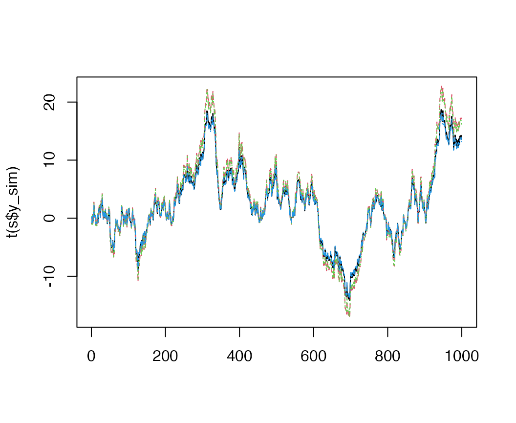
Sampling argument
In the examples below, we’ll take advantage of the
estimation argument. By default, this defaults to MCMC
(“sampling”) but can be a few other options described below. If you want
to construct a model object, but do no sampling, you can also set this
to “none”.
fit <- fit_dfa(..., estimation = "sampling")Posterior optimization
The fastest estimation approach is to do optimze the posterior (this is similar to maximum likelihood but also involves the prior distribution). We can implement this with by setting the estimation argument to “optimizing”
Note – because this model has a lot of parameters, estimation can be finicky, and can get stuck in local minima. You may have to start this from several seeds to get the model to converge successfully – or if there is a mismatch between the model and data, it may not converge at all.
For example, this model does not converge
## Warning in .local(object, ...): non-zero return code in optimizingThe optimizing output is saved here (value = log
posterior, par = estimated parameters)
names(m$model)## [1] "par" "value" "return_code" "theta_tilde"And if convergence is successful, the optimizer code will be 0 (this model isn’t converging)
m$model$return_code## [1] 70But if we change the seed, the model will converge ok:
m$model$return_code## [1] 0Posterior approximation
A second approach to quickly estimating parameters is to use
Variational Bayes, which is also implemented in Stan. This is
implemented by changing the estimation to “vb”, as shown
below. Note: this gives a helpful message that the maximum number of
iterations has been reached, so these results should not be trusted.
m <- fit_dfa(y = s$y_sim, estimation = "vb", seed=123)There are a number of other arguments that can be passed into
rstan::vb(). These include iter (maximum
iterations, defaults to 10000), tol_rel_obj (convergence
tolerance, defaults to 0.01), and output_samples (posterior
samples to save, defaults to 1000). To use these, a function call would
be
m <- fit_dfa(y = s$y_sim, estimation = "vb", seed=123, iter=20000,
             tol_rel_obj = 0.005, output_samples = 2000)