Examples of including covariates with bayesdfa

Here we will walk through how to use the bayesdfa package to fit dynamic factor analysis (DFA) models with covariates.

Let’s load the necessary packages:

library(bayesdfa)
library(ggplot2)
library(dplyr)
library(rstan)
chains = 1
iter = 10

Notation review for DFA models

Covariates in dynamic factor analysis are generally included in the observation model, rather than the process model. Without covariates, the model can be expressed as

\[{x}_{t}={x}_{t-1}+{e}_t\\ { e }_{ t }\sim MVN(0,\textbf{Q})\\ { y }_{ t }=\textbf{Z}{ x }_{ t }+{ v }_{ t }\\ { v }_{ t }\sim MVN(0,\textbf{R})\]

where the matrix \(\textbf{Z}\) is dimensioned as the number of time series by number of trends, and maps the observed data \(y_{t}\) to the latent trends \(x_{t}\).

Observation covariates

Observation covariates can be \[{x}_{t}={x}_{t-1}+{e}_t\\ { e }_{ t }\sim MVN(0,\textbf{Q})\\ { y }_{ t }=\textbf{Z}{ x }_{ t }+\textbf{D}{ d }_{ t }+{ v }_{ t }\\ { v }_{ t }\sim MVN(0,\textbf{R})\] where the matrix \(\textbf{D}\) represents time series by number of covariates at time \(t\). For a single covariate, such as temperature, this would mean estimating \(P\) parameters, where \(P\) is the number of time series. For a model including 2 covariates, the number of estimated coefficients would be \(2P\) and so forth.

Process covariates

Process covariates on the trends are less common but can be written as \[{x}_{t}={x}_{t-1}+\textbf{C}{ c }_{ t }+{e}_t\\ { e }_{ t }\sim MVN(0,\textbf{Q})\\ { y }_{ t }=\textbf{Z}{ x }_{ t }+{ v }_{ t }\\ { v }_{ t }\sim MVN(0,\textbf{R})\] where the matrix \(\textbf{C}\) represents the number of trends by number of covariates at time \(t\). For a single trend, this would mean estimating \(K\) parameters, where \(K\) is the number of trends. For a model including 2 covariates, the number of estimated coefficients would be \(2K\) and so forth.

Examples – observation covariates

We’ll start by simulating some random trends using the sim_dat function,

set.seed(1)
sim_dat <- sim_dfa(
  num_trends = 1,
  num_years = 20,
  num_ts = 4
)

Next, we can add a covariate effect to the trend estimate, x. For example,

cov = expand.grid("time"=1:20, "timeseries"=1:4, "covariate"=1)
cov$value = rnorm(nrow(cov),0,0.1)

for(i in 1:nrow(cov)) {
  sim_dat$y[cov$timeseries[i],cov$time[i]] = sim_dat$pred[cov$timeseries[i],cov$time[i]] +
  c(0.1,0.2,0.3,0.4)[cov$timeseries[i]]*cov$value[i]
}

And now fit the model with fit_dfa

mod = fit_dfa(y = sim_dat$y, obs_covar = cov, num_trends = 1,
  chains=chains, iter=iter)

We can then make plots of the true and estimated trend,

plot(c(sim_dat$x), xlab="Time", ylab="True trend")

plot_trends(rotate_trends(mod)) + ylab("Estimated trend") + theme_bw()

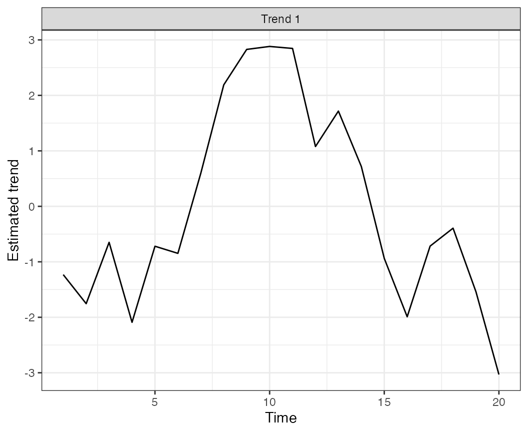
This approach could be modified to have covariates not affecting some time series. For example, if we didn’t want the covariate to affect the last time series, we could say

cov = cov[which(cov$timeseries!=4),]

And then again fit the model

mod = fit_dfa(y = sim_dat$y, obs_covar = cov, num_trends = trends,
  chains=chains)

Examples – process covariates

As a cautionary note, there’s some identifiability issues with including covariates in the process model. Covariates need to be standardized or centered prior to being included. Future versions of this vignette will include more clear examples and recommendations.