Estimating process trend variability with bayesdfa
Eric J. Ward, Sean C. Anderson, Mary E. Hunsicker, Mike A. Litzow, Luis A. Damiano, Mark D. Scheuerell, Elizabeth E. Holmes, Nick Tolimieri
2026-05-26
Source:vignettes/a5_estimate_process_sigma.Rmd
a5_estimate_process_sigma.RmdA constraint of most DFA models is that the latent trends are modeled as random walks with fixed standard deviations (= 1). We can evaluate the ability to estimate these parameters in a Bayesian context below.
Let’s load the necessary packages:
Case 1: unequal trend variability
First, let’s simulate some data. We will use the built-in function
sim_dfa(), but normally you would start with your own data.
We will simulate 20 data points from 4 time series, generated from 2
latent processes. For this first dataset, the data won’t include
extremes, and loadings will be randomly assigned (default).
We’ll tweak the default code though to model slightly different random walks, with different standard deviations for each trend. We’ll assume these standard deviations are 0.3 and 0.5, respectively.
set.seed(1)
sim_dat$x[1,] = cumsum(rnorm(n=ncol(sim_dat$x), 0, 0.1))
sim_dat$x[2,] = cumsum(rnorm(n=ncol(sim_dat$x), 0, 1))
Looking at the random walks, we can see the 2nd trend (red dashed line) is more variable than the black line.
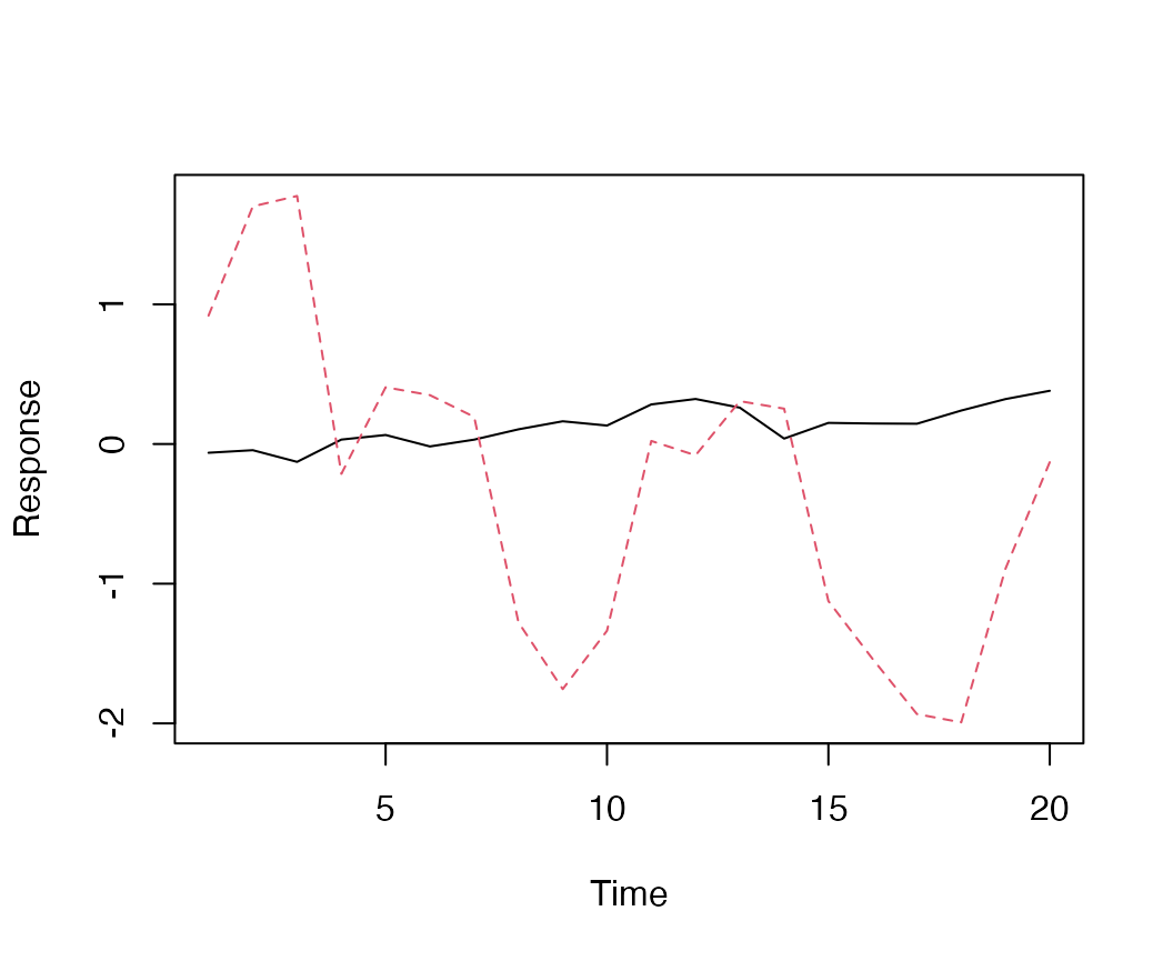
Simulated data, from a model with 2 latent trends and no extremes.
Next, we’ll calculate the predicted values of each time series and add observation error
sim_dat$pred = sim_dat$Z %*% sim_dat$x
for(i in 1:nrow(sim_dat$pred)) {
  for(j in 1:ncol(sim_dat$pred)) {
    sim_dat$y_sim[i,j] = sim_dat$pred[i,j] + rnorm(1,0,0.1)
  }
}
Candidate models
Next, we’ll fit a 2-trend DFA model to the simulated time series
using the fit_dfa() function. This default model fixed the
variances of the trends at 1 – and implicitly assumes that they have
equal variance.
f1 <- fit_dfa(
  y = sim_dat$y_sim, num_trends = 2, scale="zscore",
  iter = iter, chains = chains, thin = 1
)
r1 <- rotate_trends(f1)
Next, we’ll fit the model with process errors being estimated – and assume unequal variances by trend.
f2 <- fit_dfa(
  y = sim_dat$y_sim, num_trends = 2, scale="zscore", estimate_process_sigma = TRUE,
  equal_process_sigma = FALSE,
  iter = iter, chains = chains, thin = 1
)
r2 <- rotate_trends(f2)
Third, we’ll fit the model with process errors being estimated, unequal variances by trend, and not z-score the data (this is just a test of the scaling).
f3 <- fit_dfa(
  y = sim_dat$y_sim, num_trends = 2, scale="center", estimate_process_sigma = TRUE,
  equal_process_sigma = FALSE,
  iter = iter, chains = chains, thin = 1
)
r3 <- rotate_trends(f3)
Our fourth and fifth models will be the same as # 2 and # 3, but will estimate a single variance for both trends.
f4 <- fit_dfa(
  y = sim_dat$y_sim, num_trends = 2, scale="zscore", estimate_process_sigma = TRUE,
  equal_process_sigma = TRUE,
  iter = iter, chains = chains, thin = 1
)
r4 <- rotate_trends(f4)

f5 <- fit_dfa(
  y = sim_dat$y_sim, num_trends = 2, scale="center", estimate_process_sigma = TRUE,
  equal_process_sigma = TRUE,
  iter = iter, chains = chains, thin = 1
)
r5 <- rotate_trends(f5)
Recovering loadings
As a reminder, let’s look at the loadings from the original simulation model
##       [,1]  [,2]
## [1,]  0.57  0.00
## [2,] -0.14  0.33
## [3,]  1.18  1.06
## [4,] -1.52 -0.30
The estimated loadings from the DFA where the trends are forced to have the same fixed variance are good
##        [,1]    [,2]
## [1,] -91.70  -32.20
## [2,] -10.27 -109.07
## [3,]  42.34  -12.66
## [4,] -28.00   -7.90
but some of the loadings are far off. These loadings are also not well estimated for either of the models that estimate the process variances,
##        [,1]    [,2]
## [1,] -70.20   68.36
## [2,] -14.61 -118.64
## [3,] -66.64    9.32
## [4,] -47.34  -10.62
or
##         [,1]   [,2]
## [1,]  -92.62  37.23
## [2,] -100.07 -64.45
## [3,]   -3.13 -44.88
## [4,]  -83.12 -29.19
The loadings for Model 4 are given by
##        [,1]   [,2]
## [1,] -99.51   5.65
## [2,]  -7.46 -98.49
## [3,]   8.32   2.71
## [4,]   1.16   0.06
and Model 5 by
##        [,1]    [,2]
## [1,] -89.54  -26.98
## [2,] -19.58 -107.16
## [3,]  44.17   66.35
## [4,] -47.99  -90.43
If we calculate the RMSE of the different models, model # 3 (estimated process trends, raw data not standardized) performs the best
| Model | RMSE-loadings |
|---|---|
| 1 | 24263.24 |
| 2 | 30917.61 |
| 3 | 33873.93 |
| 4 | 19927.94 |
| 5 | 37172.58 |
Recovering trends
Let’s do the same kind of summary with the trends
| Model | RMSE-trends |
|---|---|
| 1 | 321.8506 |
| 2 | 199.0063 |
| 3 | 311.6231 |
| 4 | 128.4473 |
| 5 | 320.6021 |
These show that model 3 (trend variances are estimated, with data not standardized) performs best
Summary
In this example, the estimation model that treated the variances of the random walks as parameters performed better than models that didn’t. A caveat is that we simulated the random walk variances to be an order of magnitude difference between the 2 trends, more similar trends would need additional simulations and more thorough validation studies. Similarly, we found that not standardizing the raw time series data (instead, just centering each time series) yielded estimates of the loadings and estimated trends that were more similar to those in the simulation model. Standardizing each time series a priori yields slightly worse estimates of the trends and loadings (comparing models 2 v 3 and 4 v 5).