Simulate from a DFA
sim_dfa(
  num_trends = 1,
  num_years = 20,
  num_ts = 4,
  loadings_matrix = matrix(nrow = num_ts, ncol = num_trends, rnorm(num_ts * num_trends,
    0, 1)),
  sigma = rlnorm(1, meanlog = log(0.2), 0.1),
  varIndx = rep(1, num_ts),
  trend_model = c("rw", "bs"),
  spline_weights = matrix(ncol = 6, nrow = num_trends, data = rnorm(6 * num_trends)),
  extreme_value = NULL,
  extreme_loc = NULL,
  nu_fixed = 100,
  user_supplied_deviations = NULL
)
Arguments
- num_trends
The number of trends.
- num_years
The number of years.
- num_ts
The number of timeseries.
- loadings_matrix
A loadings matrix. The number of rows should match the number of timeseries and the number of columns should match the number of trends. Note that this loadings matrix will be internally manipulated by setting some elements to 0 and constraining some elements to 1 so that the model can be fitted. See
fit_dfa(). See the outfit elementZin the returned list is to see the manipulated loadings matrix. If not specified, a random matrix~ N(0, 1)is used.- sigma
A vector of standard deviations on the observation error. Should be of the same length as the number of trends. If not specified, random numbers are used
rlnorm(1, meanlog = log(0.2), 0.1).- varIndx
Indices of unique observation variances. Defaults to
c(1, 1, 1, 1). Unique observation error variances would be specified asc(1, 2, 3, 4)in the case of 4 time series.- trend_model
The type of trend model. Random walk (
"rw") or basis spline ("bs")- spline_weights
A matrix of basis function weights that is used if
trend_model = "bs". The number of columns should correspond to the number of knots and the number of rows should correspond to the number of trends.- extreme_value
Value added to the random walk in the extreme time step. Defaults to not included.
- extreme_loc
Location of single extreme event in the process. The same for all processes, and defaults to
round(n_t/2)wheren_tis the time series length- nu_fixed
Nu is the degrees of freedom parameter for the t-distribution, defaults to 100, which is effectively normal.
- user_supplied_deviations
An optional matrix of deviations for the trend random walks. Columns are for trends and rows are for each time step.
Value
A list with the following elements: y_sim is the simulated data,
pred is the true underlying data without observation error added, x is
the underlying trends, Z is the manipulated loadings matrix that is fed
to the model.
Examples
x <- sim_dfa(num_trends = 2)
names(x)
#> [1] "y_sim" "pred" "x" "Z" "sigma"
matplot(t(x$y_sim), type = "l")
 matplot(t(x$x), type = "l")
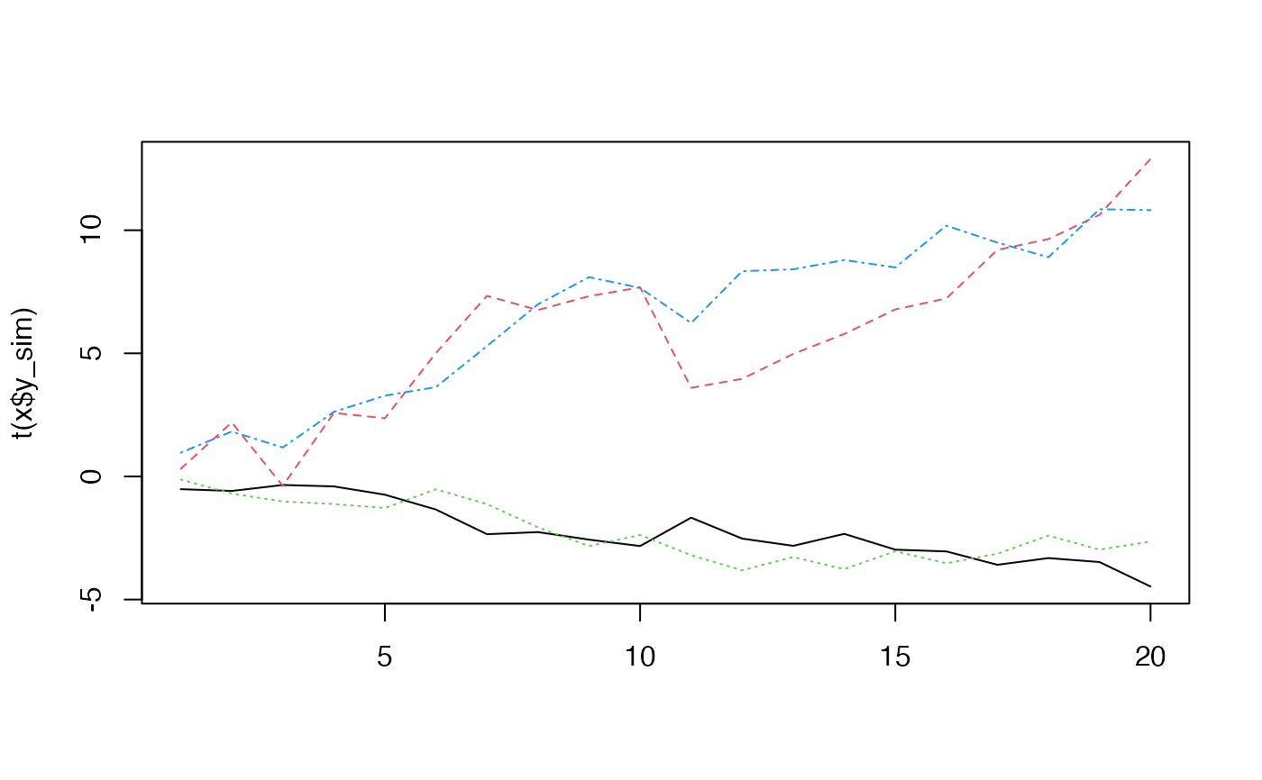
 set.seed(42)
x <- sim_dfa(extreme_value = -4, extreme_loc = 10)
matplot(t(x$x), type = "l")
abline(v = 10)
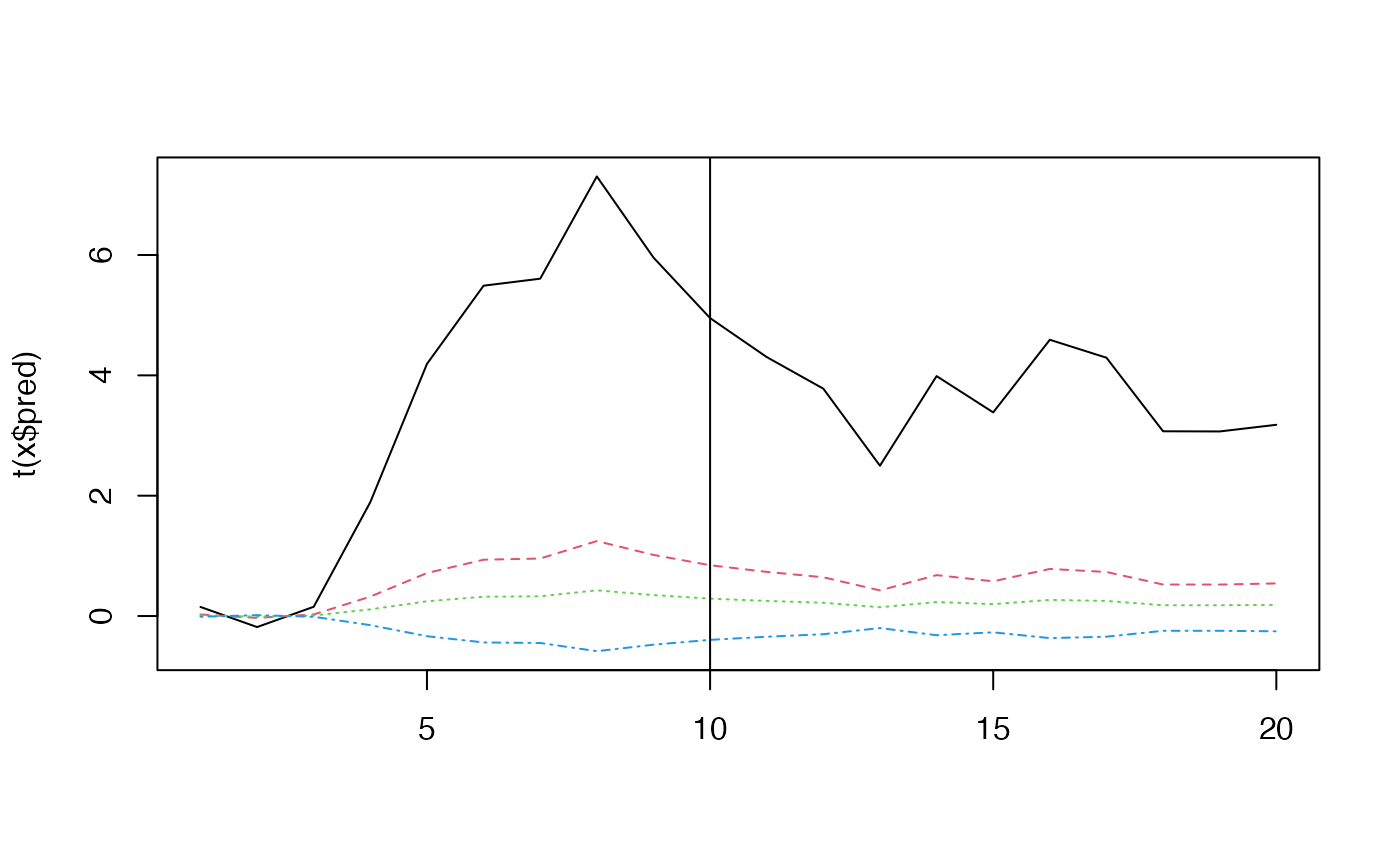
set.seed(42)
x <- sim_dfa(extreme_value = -4, extreme_loc = 10)
matplot(t(x$x), type = "l")
abline(v = 10)
 matplot(t(x$pred), type = "l")
abline(v = 10)
matplot(t(x$pred), type = "l")
abline(v = 10)
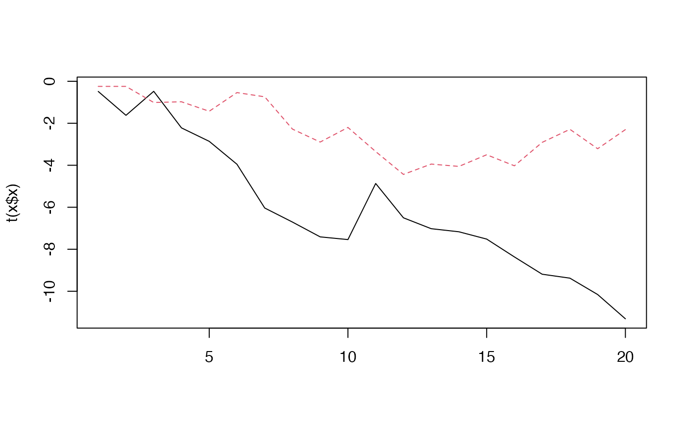
 set.seed(42)
x <- sim_dfa()
matplot(t(x$x), type = "l")
abline(v = 10)
set.seed(42)
x <- sim_dfa()
matplot(t(x$x), type = "l")
abline(v = 10)
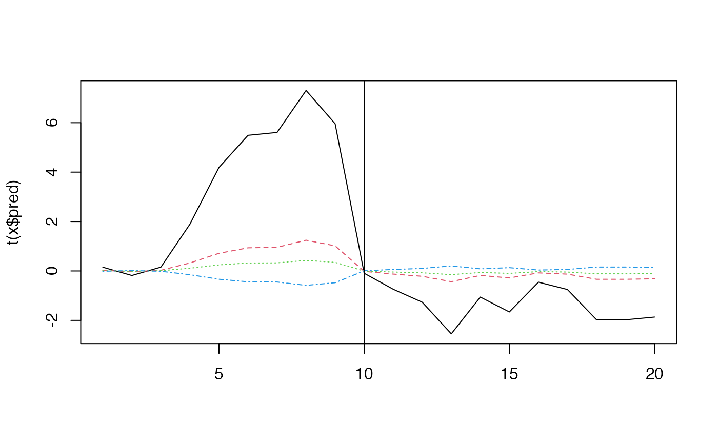
 matplot(t(x$pred), type = "l")
abline(v = 10)
matplot(t(x$pred), type = "l")
abline(v = 10)