Examples of fitting smooth trend DFA models

Eric J. Ward, Sean C. Anderson, Mary E. Hunsicker, Mike A. Litzow, Luis A. Damiano, Mark D. Scheuerell, Elizabeth E. Holmes, Nick Tolimieri

2024-10-20

In addition to fitting conventional DFA models with trends modeled as random walks (or ARMA processes), we can also construct models where underlying trends are treated as smooth trends (B-splines, P-splines, or Gaussian processes).

Let’s load the necessary packages:

library(bayesdfa)
library(ggplot2)
library(dplyr)
library(rstan)
chains = 1
iter = 10

Data simulation

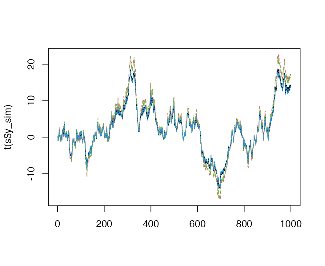
The sim_dfa function normally simulates loadings \(\sim N(0,1)\), but here we will simulate time series that are more similar with loadings \(\sim N(1,0.1)\)

set.seed(1)
s = sim_dfa(num_trends = 1, num_years = 1000, num_ts = 4,
            loadings_matrix = matrix(nrow = 4, ncol = 1, rnorm(4 * 1,
    1, 0.1)), sigma=0.05)

matplot(t(s$y_sim), type="l")

Estimating trends as B-splines

As a first approach, we can fit models where trends are estimated as B-splines. To do this, we change the trend_model argument, and specify the number of knots. More knots translates to smoother functions. For example,

set.seed(1)
fit = fit_dfa(y = s$y_sim, num_trends = 1, 
              trend_model = "bs", n_knots = 7)

Or for a model with more knots,

set.seed(1)
fit = fit_dfa(y = s$y_sim, num_trends = 1, 
              trend_model = "bs", n_knots = 14)

Estimating trends as P-splines

Obviously, trends from the B-spline model are sensitive to the number of knots. As an alternative, we also allow trends to be modeled as penalized regression splines (“P-splines”). These methods are less sensitive to the numbers of knots, and only require the knots to be enough to adequately describe the wiggliness of the function.

We can fit these kinds of models by changing the trend_model argument

set.seed(1)
fit = fit_dfa(y = s$y_sim, num_trends = 1, 
              trend_model = "ps", n_knots = 7)

Estimating trends as Gaussian processes

Finally, another type of smoothing that can be done is treating the trends as Gaussian processes. Both full rank models (knots = time points) or predictive process models may be fit (fewer knots results in smoother functions). These types of models may be specified by again changing the trend_model argument,

set.seed(1)
fit = fit_dfa(y = s$y_sim, num_trends = 1, 
              trend_model = "gp", n_knots = 7)

Comparing approaches

All of the smooth trend methods are flexible and able to capture the wiggliness of latent trends. Based on our experience, the B-spline and P-spline models will generally fit faster than the Gaussian predicitve process models (because they omit a critical matrix inversion step). The full rank Gaussian process models tend to be faster than the predictive process models. All of these approaches can be compared using cross validation, or similar predictive performance criterion.