Plot the loadings from a DFA
plot_loadings(
  rotated_modelfit,
  names = NULL,
  facet = TRUE,
  violin = TRUE,
  conf_level = 0.95,
  threshold = NULL
)
Arguments
- rotated_modelfit
Output from
rotate_trends().- names
An optional vector of names for plotting the loadings.
- facet
Logical. Should there be a separate facet for each trend? Defaults to
TRUE.- violin
Logical. Should the full posterior densities be shown as a violin plot? Defaults to
TRUE.- conf_level
Confidence level for credible intervals. Defaults to 0.95.
- threshold
Numeric (0-1). Optional for plots, if included, only plot loadings who have Pr(<0) or Pr(>0) > threshold. For example
threshold = 0.8would only display estimates where 80% of posterior density was above/below zero. Defaults toNULL(not used).
See also
plot_trends fit_dfa rotate_trends
Examples
set.seed(42)
s <- sim_dfa(num_trends = 2, num_ts = 4, num_years = 10)
# only 1 chain and 180 iterations used so example runs quickly:
m <- fit_dfa(y = s$y_sim, num_trends = 2, iter = 50, chains = 1)
#>
#> SAMPLING FOR MODEL 'dfa' NOW (CHAIN 1).
#> Chain 1:
#> Chain 1: Gradient evaluation took 1.7e-05 seconds
#> Chain 1: 1000 transitions using 10 leapfrog steps per transition would take 0.17 seconds.
#> Chain 1: Adjust your expectations accordingly!
#> Chain 1:
#> Chain 1:
#> Chain 1: WARNING: There aren't enough warmup iterations to fit the
#> Chain 1: three stages of adaptation as currently configured.
#> Chain 1: Reducing each adaptation stage to 15%/75%/10% of
#> Chain 1: the given number of warmup iterations:
#> Chain 1: init_buffer = 3
#> Chain 1: adapt_window = 20
#> Chain 1: term_buffer = 2
#> Chain 1:
#> Chain 1: Iteration: 1 / 50 [ 2%] (Warmup)
#> Chain 1: Iteration: 5 / 50 [ 10%] (Warmup)
#> Chain 1: Iteration: 10 / 50 [ 20%] (Warmup)
#> Chain 1: Iteration: 15 / 50 [ 30%] (Warmup)
#> Chain 1: Iteration: 20 / 50 [ 40%] (Warmup)
#> Chain 1: Iteration: 25 / 50 [ 50%] (Warmup)
#> Chain 1: Iteration: 26 / 50 [ 52%] (Sampling)
#> Chain 1: Iteration: 30 / 50 [ 60%] (Sampling)
#> Chain 1: Iteration: 35 / 50 [ 70%] (Sampling)
#> Chain 1: Iteration: 40 / 50 [ 80%] (Sampling)
#> Chain 1: Iteration: 45 / 50 [ 90%] (Sampling)
#> Chain 1: Iteration: 50 / 50 [100%] (Sampling)
#> Chain 1:
#> Chain 1: Elapsed Time: 0.009 seconds (Warm-up)
#> Chain 1: 0.105 seconds (Sampling)
#> Chain 1: 0.114 seconds (Total)
#> Chain 1:
#> Warning: There were 1 chains where the estimated Bayesian Fraction of Missing Information was low. See
#> https://mc-stan.org/misc/warnings.html#bfmi-low
#> Warning: Examine the pairs() plot to diagnose sampling problems
#> Warning: The largest R-hat is NA, indicating chains have not mixed.
#> Running the chains for more iterations may help. See
#> https://mc-stan.org/misc/warnings.html#r-hat
#> Warning: Bulk Effective Samples Size (ESS) is too low, indicating posterior means and medians may be unreliable.
#> Running the chains for more iterations may help. See
#> https://mc-stan.org/misc/warnings.html#bulk-ess
#> Warning: Tail Effective Samples Size (ESS) is too low, indicating posterior variances and tail quantiles may be unreliable.
#> Running the chains for more iterations may help. See
#> https://mc-stan.org/misc/warnings.html#tail-ess
#> Inference for the input samples (1 chains: each with iter = 25; warmup = 12):
#>
#> Q5 Q50 Q95 Mean SD Rhat Bulk_ESS Tail_ESS
#> x[1,1] -1.5 -0.7 0.6 -0.6 0.7 1.37 6 13
#> x[2,1] -1.0 -0.2 0.5 -0.2 0.5 1.58 9 13
#> x[1,2] -1.7 0.0 0.9 -0.4 1.1 1.87 4 13
#> x[2,2] 0.2 0.5 1.2 0.6 0.4 1.00 12 13
#> x[1,3] -1.6 0.0 0.9 -0.3 1.0 2.06 4 13
#> x[2,3] -1.1 -0.2 0.3 -0.4 0.5 2.06 4 13
#> x[1,4] -1.5 -0.4 0.7 -0.4 0.9 1.87 4 13
#> x[2,4] -0.1 0.5 1.3 0.5 0.5 0.97 11 13
#> x[1,5] -0.9 -0.2 0.7 -0.1 0.6 0.95 13 13
#> x[2,5] -1.4 -0.6 1.3 -0.3 1.1 1.87 6 13
#> x[1,6] -1.1 -0.3 0.3 -0.4 0.5 1.06 7 13
#> x[2,6] -0.2 0.1 0.6 0.1 0.3 1.45 10 13
#> x[1,7] -2.2 -1.2 0.2 -1.1 0.9 1.71 4 13
#> x[2,7] -1.1 -0.1 0.9 -0.2 0.6 1.39 13 13
#> x[1,8] -1.7 -0.8 0.5 -0.6 0.8 1.32 5 13
#> x[2,8] -1.5 0.2 1.4 0.1 0.9 1.87 13 13
#> x[1,9] -1.1 -0.2 0.7 -0.2 0.6 1.15 8 13
#> x[2,9] -1.3 0.5 1.2 0.1 0.9 2.06 9 13
#> x[1,10] -1.4 -0.7 0.2 -0.7 0.6 1.58 4 13
#> x[2,10] -1.0 -0.4 0.3 -0.5 0.4 0.99 13 13
#> Z[1,1] -3.6 0.6 3.6 0.3 2.4 2.06 13 13
#> Z[2,1] -0.5 0.5 1.4 0.3 0.7 0.95 13 13
#> Z[3,1] -1.5 -0.5 1.3 -0.3 1.0 1.87 4 13
#> Z[4,1] -0.8 0.1 1.9 0.4 0.9 1.25 5 13
#> Z[1,2] 0.0 0.0 0.0 0.0 0.0 1.00 13 13
#> Z[2,2] -4.2 0.5 6.2 0.5 3.9 1.58 13 13
#> Z[3,2] -1.6 -0.7 0.5 -0.6 0.8 1.01 10 13
#> Z[4,2] -1.2 0.8 1.5 0.5 1.0 0.97 13 13
#> log_lik[1] -4.3 -1.5 -0.7 -2.1 1.4 1.87 4 13
#> log_lik[2] -4.3 -1.3 -0.6 -1.9 1.4 1.87 4 13
#> log_lik[3] -4.3 -1.3 -0.8 -2.0 1.4 2.06 4 13
#> log_lik[4] -4.3 -1.1 -0.6 -2.0 1.5 2.06 4 13
#> log_lik[5] -4.3 -1.5 -0.8 -2.1 1.4 1.87 4 13
#> log_lik[6] -4.3 -1.3 -0.8 -2.1 1.4 1.71 4 13
#> log_lik[7] -4.3 -1.3 -0.8 -2.0 1.4 1.87 4 13
#> log_lik[8] -4.7 -1.4 -0.6 -2.4 1.7 1.87 4 13
#> log_lik[9] -4.6 -3.5 -2.2 -3.3 1.0 0.91 12 13
#> log_lik[10] -4.3 -2.3 -1.1 -2.7 1.2 1.10 8 13
#> log_lik[11] -4.3 -2.1 -0.6 -2.5 1.4 1.32 4 13
#> log_lik[12] -4.3 -1.6 -0.8 -2.2 1.3 1.38 4 13
#> log_lik[13] -4.3 -1.4 -0.8 -2.1 1.4 1.87 4 13
#> log_lik[14] -4.3 -1.5 -0.7 -2.0 1.4 1.87 4 13
#> log_lik[15] -4.3 -1.5 -0.6 -2.0 1.4 2.06 4 13
#> log_lik[16] -4.3 -1.5 -0.8 -2.3 1.4 1.87 4 13
#> log_lik[17] -4.3 -1.3 -0.6 -1.9 1.5 2.06 4 13
#> log_lik[18] -4.4 -2.0 -0.7 -2.2 1.4 2.06 4 13
#> log_lik[19] -4.3 -1.9 -0.6 -2.1 1.4 2.06 4 13
#> log_lik[20] -4.3 -1.7 -0.7 -2.1 1.3 2.06 4 13
#> log_lik[21] -4.3 -1.1 -0.5 -1.9 1.5 2.06 3 13
#> log_lik[22] -4.3 -1.2 -0.6 -1.8 1.5 2.06 4 13
#> log_lik[23] -4.3 -2.1 -0.7 -2.1 1.4 1.47 4 13
#> log_lik[24] -4.3 -1.3 -0.6 -1.9 1.5 2.06 4 13
#> log_lik[25] -4.4 -2.2 -0.7 -2.4 1.6 1.71 4 13
#> log_lik[26] -4.3 -1.5 -0.7 -2.0 1.4 1.58 4 13
#> log_lik[27] -4.3 -1.6 -0.8 -2.1 1.4 2.06 4 13
#> log_lik[28] -4.3 -1.6 -0.8 -2.1 1.4 1.87 4 13
#> log_lik[29] -4.3 -1.5 -0.7 -2.2 1.3 1.47 4 13
#> log_lik[30] -4.3 -1.3 -0.6 -1.9 1.4 1.71 4 13
#> log_lik[31] -4.3 -1.1 -0.5 -1.8 1.5 2.06 3 13
#> log_lik[32] -4.3 -1.4 -0.8 -2.0 1.3 1.87 4 13
#> log_lik[33] -4.3 -1.6 -0.9 -2.2 1.3 1.71 4 13
#> log_lik[34] -4.3 -1.6 -0.6 -2.1 1.4 2.06 4 13
#> log_lik[35] -4.3 -1.0 -0.5 -1.8 1.5 2.06 4 13
#> log_lik[36] -4.3 -1.0 -0.7 -1.9 1.5 2.06 4 13
#> log_lik[37] -4.3 -2.0 -0.7 -2.2 1.4 1.87 4 13
#> log_lik[38] -4.3 -1.2 -0.6 -1.9 1.5 2.06 3 13
#> log_lik[39] -4.3 -1.5 -0.9 -2.1 1.3 1.71 4 13
#> log_lik[40] -4.3 -1.2 -0.6 -1.9 1.4 2.06 4 13
#> xstar[1,1] -2.0 -1.1 1.3 -0.7 1.2 0.95 10 13
#> xstar[2,1] -1.7 -0.4 1.2 -0.3 1.1 1.25 6 13
#> sigma[1] 0.7 1.0 29.7 7.5 11.7 2.06 4 13
#> lp__ -203.1 -43.1 -22.2 -79.4 72.4 2.06 3 13
#>
#> For each parameter, Bulk_ESS and Tail_ESS are crude measures of
#> effective sample size for bulk and tail quantities respectively (an ESS > 100
#> per chain is considered good), and Rhat is the potential scale reduction
#> factor on rank normalized split chains (at convergence, Rhat <= 1.05).
r <- rotate_trends(m)
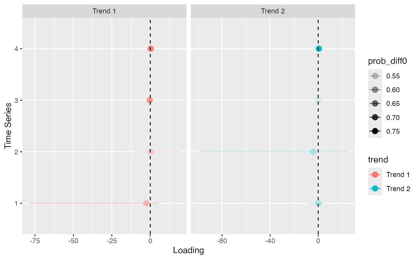
plot_loadings(r, violin = FALSE, facet = TRUE)
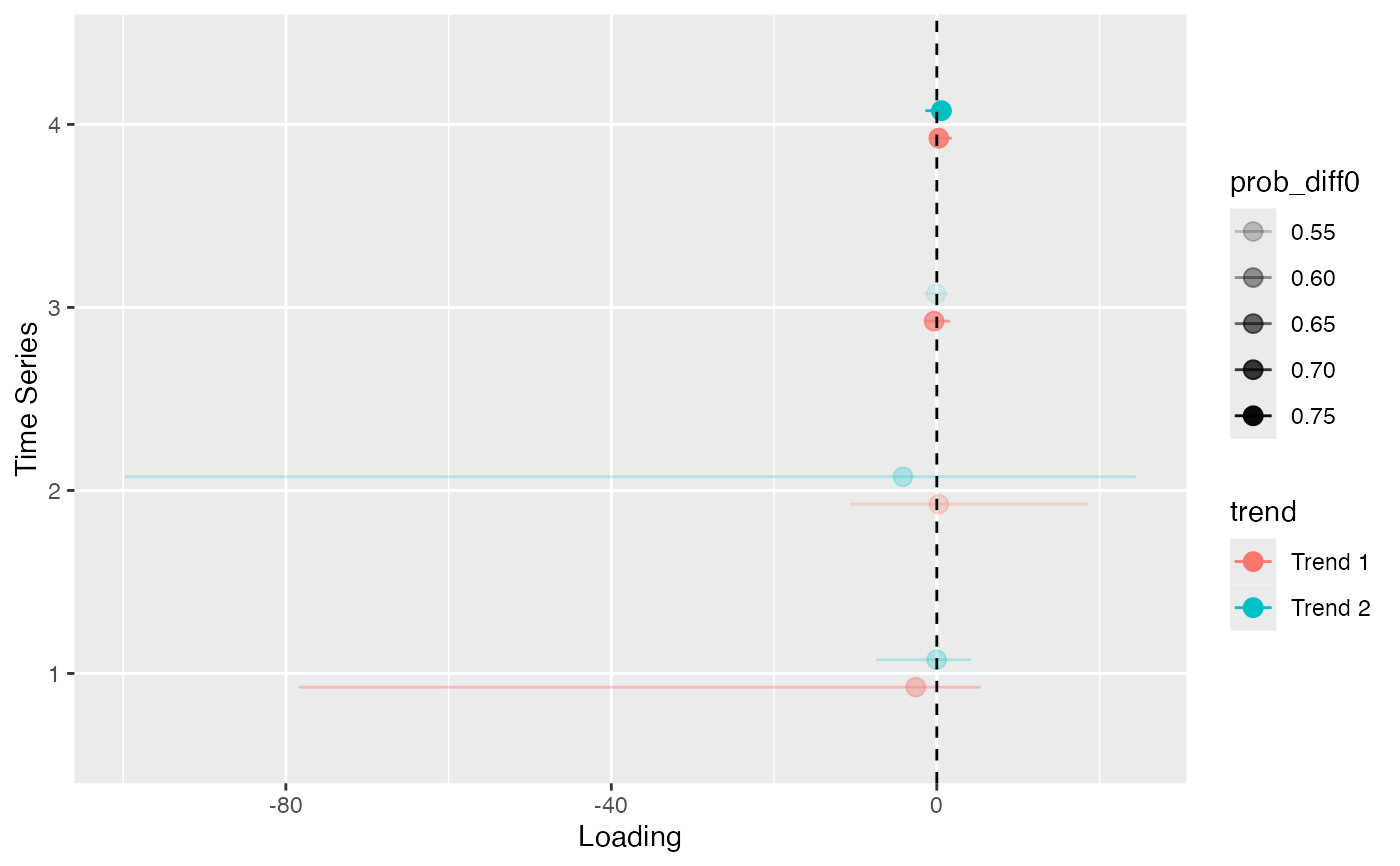
 plot_loadings(r, violin = FALSE, facet = FALSE)
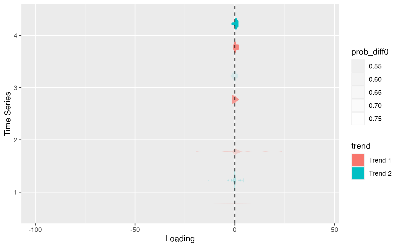
 plot_loadings(r, violin = TRUE, facet = FALSE)
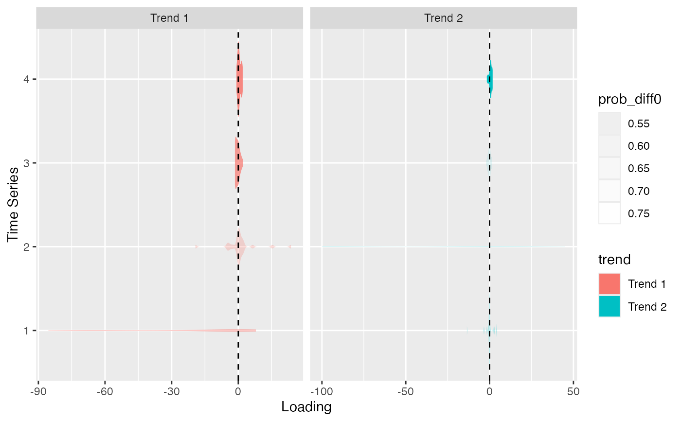
 plot_loadings(r, violin = TRUE, facet = TRUE)