Plot the state probabilities from find_regimes()

Plot the state probabilities from find_regimes()

plot_regime_model(
  model,
  probs = c(0.05, 0.95),
  type = c("probability", "means"),
  regime_prob_threshold = 0.9,
  plot_prob_indices = NULL,
  flip_regimes = FALSE
)

Arguments

model

A model returned by find_regimes().

probs

A numeric vector of quantiles to plot the credible intervals at. Defaults to c(0.05, 0.95).

type

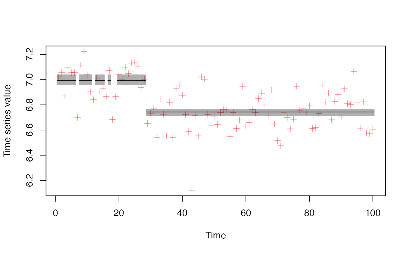
Whether to plot the probabilities (default) or means.

regime_prob_threshold

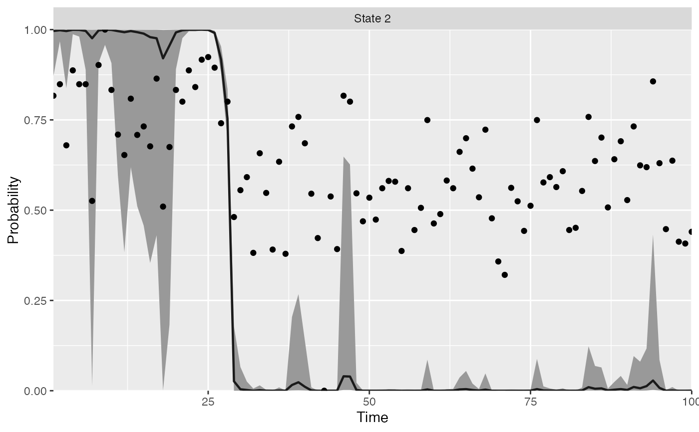
The probability density that must be above 0.5. Defaults to 0.9 before we classify a regime (only affects "means" plot).

plot_prob_indices

Optional indices of probability plots to plot. Defaults to showing all.

flip_regimes

Optional whether to flip regimes in plots, defaults to FALSE

Details

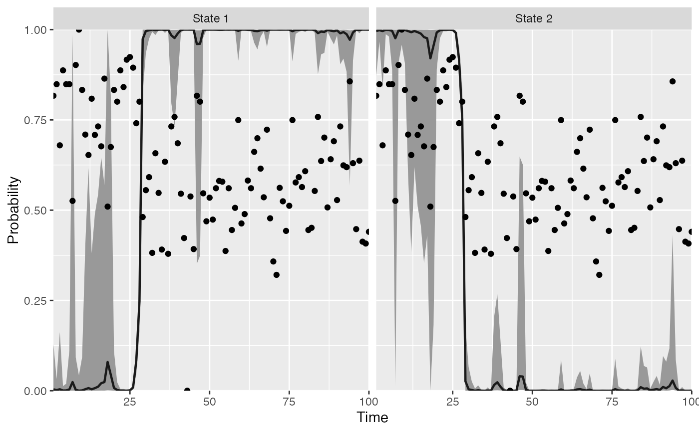
Note that the original timeseries data (dots) are shown scaled between 0 and 1.

Examples

# \donttest{
data(Nile)
m <- fit_regimes(log(Nile), n_regimes = 2, chains = 1, iter = 50)
#> 
#> SAMPLING FOR MODEL 'hmm_gaussian' NOW (CHAIN 1).
#> Chain 1: 
#> Chain 1: Gradient evaluation took 0.000101 seconds
#> Chain 1: 1000 transitions using 10 leapfrog steps per transition would take 1.01 seconds.
#> Chain 1: Adjust your expectations accordingly!
#> Chain 1: 
#> Chain 1: 
#> Chain 1: WARNING: There aren't enough warmup iterations to fit the
#> Chain 1:          three stages of adaptation as currently configured.
#> Chain 1:          Reducing each adaptation stage to 15%/75%/10% of
#> Chain 1:          the given number of warmup iterations:
#> Chain 1:            init_buffer = 3
#> Chain 1:            adapt_window = 20
#> Chain 1:            term_buffer = 2
#> Chain 1: 
#> Chain 1: Iteration:  1 / 50 [  2%]  (Warmup)
#> Chain 1: Iteration:  5 / 50 [ 10%]  (Warmup)
#> Chain 1: Iteration: 10 / 50 [ 20%]  (Warmup)
#> Chain 1: Iteration: 15 / 50 [ 30%]  (Warmup)
#> Chain 1: Iteration: 20 / 50 [ 40%]  (Warmup)
#> Chain 1: Iteration: 25 / 50 [ 50%]  (Warmup)
#> Chain 1: Iteration: 26 / 50 [ 52%]  (Sampling)
#> Chain 1: Iteration: 30 / 50 [ 60%]  (Sampling)
#> Chain 1: Iteration: 35 / 50 [ 70%]  (Sampling)
#> Chain 1: Iteration: 40 / 50 [ 80%]  (Sampling)
#> Chain 1: Iteration: 45 / 50 [ 90%]  (Sampling)
#> Chain 1: Iteration: 50 / 50 [100%]  (Sampling)
#> Chain 1: 
#> Chain 1:  Elapsed Time: 0.295 seconds (Warm-up)
#> Chain 1:                0.362 seconds (Sampling)
#> Chain 1:                0.657 seconds (Total)
#> Chain 1: 
#> Warning: The largest R-hat is NA, indicating chains have not mixed.
#> Running the chains for more iterations may help. See
#> https://mc-stan.org/misc/warnings.html#r-hat
#> Warning: Bulk Effective Samples Size (ESS) is too low, indicating posterior means and medians may be unreliable.
#> Running the chains for more iterations may help. See
#> https://mc-stan.org/misc/warnings.html#bulk-ess
#> Warning: Tail Effective Samples Size (ESS) is too low, indicating posterior variances and tail quantiles may be unreliable.
#> Running the chains for more iterations may help. See
#> https://mc-stan.org/misc/warnings.html#tail-ess
#> Warning: Some Pareto k diagnostic values are too high. See help('pareto-k-diagnostic') for details.
plot_regime_model(m)

plot_regime_model(m, plot_prob_indices = c(2))

plot_regime_model(m, type = "means")

# }